Acquire and visualize USGS hydrology data in Python
Climata is a python package aimed at acquiring climate and water flow data from a variety of organizations including NOAA, CoCoRaHS, USBR, NWS, NRCS, and USGS. Here, we’ll use climata to acquire streamflow data in and around Boulder, Colorado.
Objectives
- Extracting stream flow data for a specific USGS station ID
- Extracting stream flow data for a county by FIPS code
Dependencies
This is climata running in Python 3.4. Many data queries are possible through climata, some of which are demonstrated here.
import matplotlib
import matplotlib.pyplot as plt
from climata.usgs import DailyValueIO
import pandas as pd
import numpy as np

plt.style.use('ggplot')
%matplotlib inline
matplotlib.rcParams['figure.figsize'] = (14.0, 8.0)
Extracting data for a specific USGS station ID
To acquire station data, you must know which station you want to access. There is a nice interactive application here to do this.
# set parameters
nyears = 10
ndays = 365 * nyears
station_id = "06730200"
param_id = "00060"

datelist = pd.date_range(end=pd.datetime.today(), periods=ndays).tolist()
data = DailyValueIO(
    start_date=datelist[0],
    end_date=datelist[-1],
    station=station_id,
    parameter=param_id,
)
# create lists of date-flow values
for series in data:
    flow = [r[0] for r in series.data]
    dates = [r[1] for r in series.data]
plt.plot(dates, flow)
plt.xlabel('Date')
plt.ylabel(series.variable_name)
plt.title(series.site_name)
plt.xticks(rotation='vertical')
plt.margins(0.2)
plt.show()
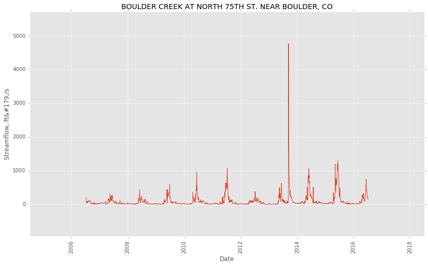
Note that the flooding in 2013 is fairly apparent.
Extracting data for a county using a FIPS code
If we want data for all stations within a county, we need to query using the county FIPS code. The FIPS code for Boulder, CO is 08013:
# set parameters
nyears = 1
ndays = 365 * nyears
county = "08013"
datelist = pd.date_range(end=pd.datetime.today(), periods=ndays).tolist()

data = DailyValueIO(
    start_date=datelist[0],
    end_date=datelist[-1],
    county=county,
)

date = []
value = []

for series in data:
    for row in series.data:
        date.append(row[1])
        value.append(row[0])
site_names = [[series.site_name] * len(series.data) for series in data]

# unroll the list of lists
flat_site_names = [item for sublist in site_names for item in sublist]
# bundle the data into a data frame
df = pd.DataFrame({'site': flat_site_names,
                   'date': date,
                   'value': value})

# remove missing values
df = df[df['value'] != -999999.0]
# visualize flow time series, coloring by site
groups = df.groupby('site')
fig, ax = plt.subplots()
for name, group in groups:
    ax.plot(group.date, np.log(group.value), marker='o', linestyle='-', ms=2, label=name)
ax.legend(bbox_to_anchor=(1.05, 1), loc=2, borderaxespad=0.)
plt.xlabel('Date')
plt.ylabel('log(' + series.variable_name + ')')
plt.xticks(rotation='vertical')
plt.margins(0.2)
plt.show()
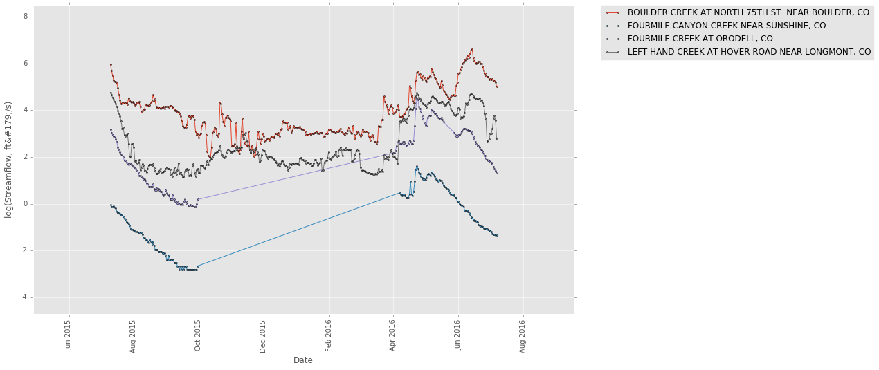
Note that there are gaps in the data, where points do not occur. Lines bridge areas lacking data.